KNN Algorithm

When do we use KNN algorithm?

KNN can be used for both classification and regression predictive problems. However, it is more widely used in classification problems in the industry. To evaluate any technique we generally look at 3 important aspects:

1. Ease to interpret output

2. Calculation time

3. Predictive Power

Let us take a few examples to  place KNN in the scale :

KNN algorithm fairs across all parameters of considerations. It is commonly used for its easy of interpretation and low calculation time.

How does the KNN algorithm work?

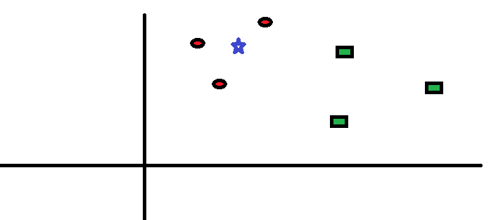
Let’s take a simple case to understand this algorithm. Following is a spread of red circles (RC) and green squares (GS) :

You intend to find out the class of the blue star (BS) . BS can either be RC or GS and nothing else. The “K” is KNN algorithm is the nearest neighbors we wish to take vote from. Let’s say K = 3. Hence, we will now make a circle with BS as center just as big as to enclose only three data points on the plane. Refer to following diagram for more details:

The three closest points to BS is all RC. Hence, with good confidence level we can say that the BS should belong to the class RC. Here, the choice became very obvious as all three votes from the closest neighbor went to RC. The choice of the parameter K is very crucial in this algorithm. Next we will understand what are the factors to be considered to conclude the best K.

How do we choose the factor K?

First let us try to understand what exactly does K influence in the algorithm. If we see the last example, given that all the 6 training observation remain constant, with a given K value we can make boundaries of each class. These boundaries will segregate RC from GS. The same way, let’s try to see the effect of value “K” on the class boundaries. Following are the different boundaries separating the two classes with different values of K.

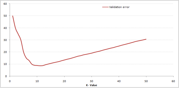
If you watch carefully, you can see that the boundary becomes smoother with increasing value of K. With K increasing to infinity it finally becomes all blue or all red depending on the total majority.  The training error rate and the validation error rate are two parameters we need to access on different K-value. Following is the curve for the training error rate with varying value of K :

As you can see, the error rate at K=1 is always zero for the training sample. This is because the closest point to any training data point is itself. Hence the prediction is always accurate with K=1. If validation error curve would have been similar, our choice of K would have been 1. Following is the validation error curve with varying value of K:

This makes the story clearer. At K=1, we were over fitting the boundaries. Hence, error rate initially decreases and reaches a minimal. After the minima point, it then increase with increasing K. To get the optimal value of K, you can segregate the training and validation from the initial dataset. Now plot the validation error curve to get the optimal value of K. This value of K should be used for all predictions.